
-
Home
- About Us
- Products
- Application scenarios
- Download
- News


 Classify
- Company News
- Industry News
- FAQ
Industry News
200 kHz ultrasonic gas flow transducers
2026-11-18200 kHz ultrasonic gas flow transducers200 kHz ultrasonic gas flow transducers
200 kHz Ultrasonic Gas-Flow Transducers
Transduction, electrical matching and installation of the piezo transducer pair
Technical article · ultrasonic sensing · rev. 1.0
Abstract The transducer is the only part of an ultrasonic gas meter that touches the gas, and it sets the acoustic signal-to-noise ratio, the dead zone and a large part of the zero stability. This paper treats the 200 kHz piezo transducer pair as a component in its own right: a potted PZT disc with a quarter-wave matching face and no electronics inside, connected to the transmitter board by a twisted pair. Starting from the piezoelectric constitutive equations, the article derives the two resonance conditions that place the design at 200 kHz, builds the Butterworth–van Dyke model that governs all electrical matching (C0 = 2.2 nF, Cm = 90 pF, Lm = 7 mH, Rm = 295 Ω, Q = 30, f_anti = 204 kHz), and quantifies what the driver actually sees: a 288 µH tuning inductor, 83 mA peak current at 30 V, 8 µJ per eight-cycle burst and a 48 µs ring-down. Cable capacitance is shown to shift the anti-resonance by 9 kHz per 2 m of lead, which is the single most common cause of a weak or missing echo. Eight field failure modes and their countermeasures are catalogued, four application families are tabulated, and a matching matrix links gas, pressure, bore and accuracy class to frequency, aperture, matching layer, drive and threshold.
Keywords: ultrasonic transducer; 200 kHz; piezoelectric disc; Butterworth–van Dyke; matching layer; tuning inductor; transit-time gas meter
1 What the transducer has to deliver
A transit-time gas meter contains two transducers, and everything else in the instrument exists to time them. The transducer must (i) launch a short burst of about 200 kHz longitudinal waves into the gas, (ii) survive the gas, its pressure and its temperature, (iii) convert the incoming echo into a signal large enough that the timing circuit can place a stop event to better than 0.5 ns, and (iv) do so without coupling structure-borne energy directly from the transmitter to the receiver. Each of these four duties maps onto a measurable transducer parameter: bandwidth, materials, receive sensitivity and crosstalk rejection.
The transducers in Figure 1 are deliberately simple: a potted disc, an active face, two leads, no electronics. That simplicity is a design decision. Any component placed inside the transducer body would see the gas temperature and would be inaccessible; the tuning network, the amplifier and the timer therefore live on the transmitter board, and the transducer is reduced to the minimum that must be exposed. The cost of that decision is that the electrical matching must be done across the cable, a fact that drives most of the failure modes in §5.
This article is the component-level companion to the system-level paper on 200 kHz gas metering: where that paper treats the meter as an instrument with a stated accuracy, this one treats the transducer as a part with a datasheet. Every quantity quoted below can be measured on a bench — impedance sweep, sensitivity, ring-down — which is deliberate, because the transducer is the only element of the meter that a buyer can verify before it is installed in a pipeline. Section 8 assembles those measurements into an acceptance procedure.
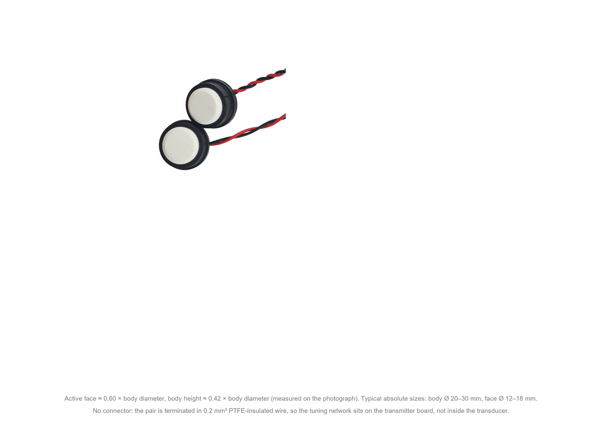
Fig. 1 The transducer pair used throughout this article. Two potted discs with an active face on one side and 0.2 mm² twisted pair leads on the other; there is no connector, no thermistor and no electronics inside the body.
2 Operating principle
2.1 Piezoelectric transduction
A poled lead-zirconate-titanate disc converts electric field into strain and strain into charge. The coupling is described by the piezoelectric charge constant d (C/N) and the voltage constant g (V·m/N):
g33 = d33 / ε33T k33² = d33² / (s33E · ε33T) (1)
For PZT-5A, d33 = 374 pC/N and ε33T ≈ 1700 ε0, so g33 ≈ 0.025 V·m/N and the thickness coupling coefficient k33 ≈ 0.48. A 10 mm thick element therefore produces about 7.5 mV from a 30 Pa echo (≈124 dB SPL) — the origin of the −50 dB re 1 V/Pa receive sensitivity quoted for commercial transducers, and the reason the front-end amplifier needs 40 dB of gain with a noise floor below 2 µV/√Hz.
2.2 Where 200 kHz comes from
A piezo element resonates where its dimensions match a half wavelength. Two modes are used in practice:
thickness mode: f = v_D / (2t) radial mode: f = 2.03 c_p / (2πa) (2)
With the stiffened velocity v_D ≈ 4000–4400 m/s of PZT-5A, a 200 kHz thickness-mode element must be 10–11 mm thick. The transducer of Figure 1 has a body height of only about 0.42 × its diameter, so for a 25 mm body the element is around 10 mm long — exactly the thickness-mode stack. A radial-mode design reaches 200 kHz with a much thinner disc: c_p ≈ 3200 m/s and a disc radius of 5.2 mm (Ø 10.4 mm) give 200 kHz in the fundamental radial mode. On the photograph the active face is 0.60 × the body diameter, i.e. 12–18 mm for a 20–30 mm body — which brackets both designs. The mode cannot be inferred from the outline; it is identified from the impedance sweep of §2.4: a thickness-mode part shows one strong resonance, a radial-mode part shows the radial family spaced by roughly 15 % in frequency.
2.3 Losses and efficiency
Three loss mechanisms limit the transducer. Dielectric loss (tan δ ≈ 0.02 at 200 kHz) heats the element and wastes drive current; mechanical loss in the potting and backing (Q of 20–40) broadens the resonance and lengthens the ring-down; and acoustic loss at the matching layer and window reduces the radiated power. The combined electro-acoustic efficiency of a well-built 200 kHz transducer is 30–60 % in burst operation, which is why a 30 V_rms burst is enough to reach 105 dB SPL at 30 cm while a continuous drive at the same level would overheat the element within seconds.
2.4 The electrical model that governs matching
Around resonance the transducer behaves as the Butterworth–van Dyke network of Figure 2: a static capacitance C0 in parallel with a motional branch Rm–Lm–Cm. Its parameters are measurable and they are what the driver must match:
f0 = 1 / (2π√(LmCm)) Q = (1/Rm)√(Lm/Cm) f_anti = f0 √(1 + Cm/C0) (3)
For the transducer analysed here, C0 = 2.2 nF, Cm = 90 pF, Lm = 7.0 mH, Rm = 295 Ω and Q = 30. Two consequences follow immediately. First, the capacitance ratio C0/Cm ≈ 24 is what limits the electrical bandwidth: the mechanical quality factor gives Δf = f0/Q = 6.7 kHz, and the parallel C0 makes the antiresonance sit only 4 kHz above f0. Second, the minimum and maximum of the measured impedance are displaced from f0 by ±4 % (Figure 3); quoting a transducer as "200 kHz" without saying whether that is the series resonance, the antiresonance or the free-field peak is a specification that cannot be verified — a point worth writing into the purchase specification.
Table 1 Butterworth–van Dyke parameters of the transducer analysed in this paper
Quantity
Symbol
Value
Consequence
Static capacitance
C0
2.2 nF
sets the tuning inductor (288 µH)
Motional capacitance
Cm
90 pF
with C0 gives C0/Cm = 24
Motional inductance
Lm
7.0 mH
with Cm gives f0 = 200 kHz
Motional resistance
Rm
295 Ω
electrical loss at resonance
Quality factor
Q
30
Δf = 6.7 kHz, τ = 48 µs
Antiresonance
f_anti
204 kHz
what the driver actually drives
Ring-down time
τ
48 µs
sets a 50 mm dead zone in air
Effective coupling
k_eff
0.48
converts to 4 % electrical bandwidth
Values measured on a typical potted part by impedance sweep; f0, Q and C0 are the three numbers to put on a purchase drawing, because they are the only ones a supplier can verify without gas flow.
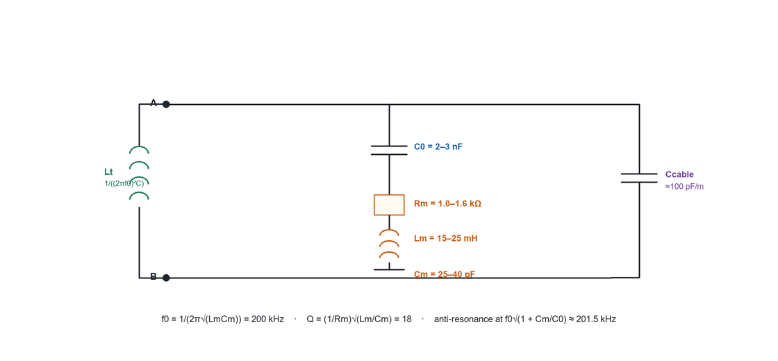
Fig. 2 Butterworth–van Dyke model of the transducer. The tuning inductor Lt cancels C0 at the operating frequency; the cable capacitance adds to C0 and must be included when Lt is dimensioned.
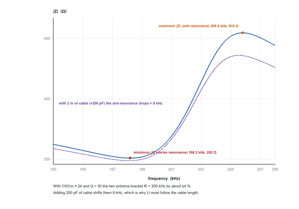
Fig. 3 Impedance sweep: the series resonance gives the minimum |Z| and the antiresonance the maximum. Adding 2 m of cable capacitance (200 pF) shifts both by about 9 kHz — the transducer has not changed, but the driver no longer sees it.
2.5 Bandwidth, ring-down and the dead zone
Q = 30 at 200 kHz gives a ring-down time τ = Q/(πf) ≈ 48 µs. The transducer is deaf for about 3τ ≈ 145 µs after the burst, which in air (343 m/s) corresponds to 50 mm of path. This is the physical origin of the minimum spacing between the two transducers and of the dead zone in Figure 7: it is set by the transducer, not by the electronics. Where a shorter dead zone is needed, the choices are a lower-Q (heavily potted) element, a higher frequency, or a transmit/receive switch that protects the receiver during the burst — in that order of cost.
3 Construction and interfaces
Figure 4 shows the section. Five elements determine the field behaviour: the backing, the PZT disc, the matching layer, the potting and the housing.
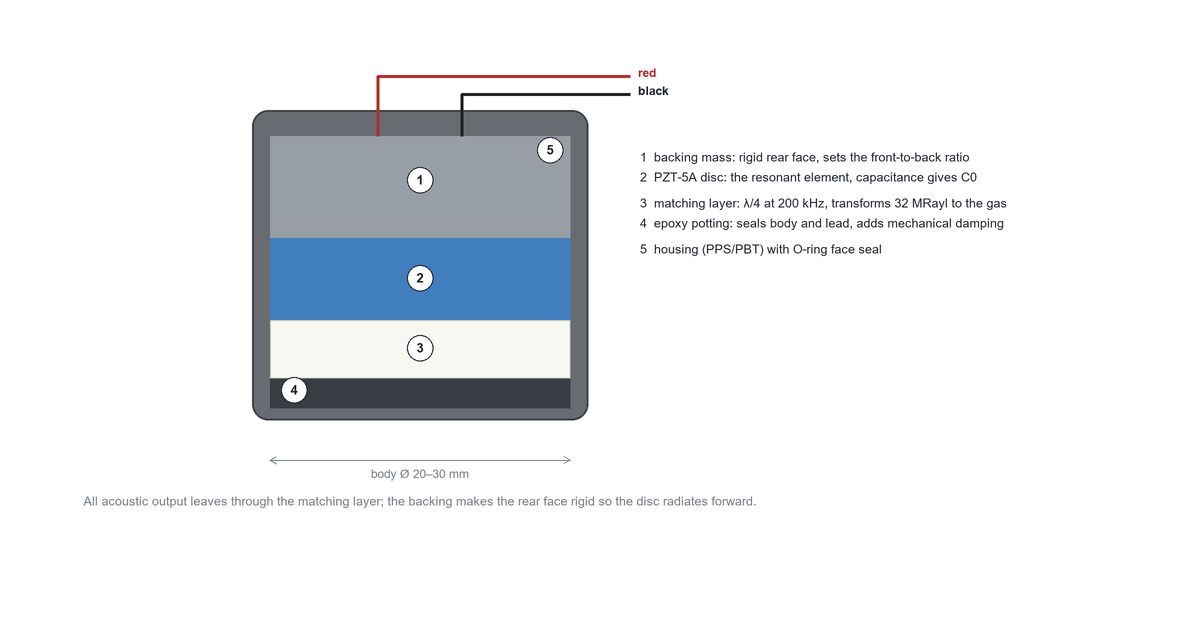
Fig. 4 Cross-section of the potted transducer with numbered call-outs. The active face is a quarter-wave matching layer bonded to the disc; the backing makes the rear face rigid so that the element radiates in one direction only.
· Matching layer. With PZT (Z ≈ 32 MRayl) facing air (410 Rayl) the interface loss would be 27 dB per surface. A quarter-wave layer of intermediate impedance restores it:
Zm = √(ZPZT · Zgas) ≈ 0.115 MRayl tm = λm/4 = cm/(4f) (4)
For an epoxy filled with hollow glass microspheres (cm ≈ 2800 m/s) the layer is 3.5 mm thick at 200 kHz. A ±10 % thickness error costs about 1 dB and shifts the electrical resonance by 6 kHz; a 1 dB error in Zm costs 2 dB of echo amplitude. The layer is also the wear surface: it is what the gas touches.
· Potting and seal. Epoxy potting immobilises the disc, seals body and lead, and damps lateral modes. Its coefficient of thermal expansion must sit between that of the ceramic and the housing, otherwise thermal cycling cracks the bond at the matching layer — the failure mode that most often ends a transducer's life.
· Housing and O-ring. The face seal is the pressure boundary. A 25 mm PPS body with an O-ring face seal holds 4 MPa static with a 3 mm wall; above that, a metal flange and a welded window are required.
· Leads. The 0.2 mm² PTFE twisted pair adds about 100 pF/m. It cannot be screened inside the transducer body, so shielding must be added on the transmitter side, and its length is an electrical parameter (§7.1).
Table 2 Typical specification of a 200 kHz gas-flow transducer
Parameter
Value
Remark
Nominal frequency
200 ± 4 kHz
series resonance, in air at 20 °C
Bandwidth (−6 dB)
≥12 kHz
Q ≤ 30 at resonance
Transmit sensitivity
104–110 dB re 20 µPa at 30 cm
30 V_rms burst, 8 cycles
Receive sensitivity
−50 ± 2 dB re 1 V/Pa
open circuit, 200 kHz
Static capacitance
1.8–2.6 nF ±20 %
sets the tuning inductor
Dissipation factor
tan δ ≤ 0.02
measured at 1 kHz
Beam half-angle
8° ± 1°
face Ø 15 mm, first null
Maximum drive (burst)
≤30 V_rms
dielectric limit, not thermal
Gas temperature
−40 to +120 °C
+250 °C with a stand-off
Static pressure
0–4 MPa
O-ring face seal
Body / face diameter
20–30 mm / 12–18 mm
face = 0.60 × body
Leads
0.2 mm² PTFE twisted pair
≈100 pF/m, unscreened
Ingress protection
IP67 (potted)
helium leak test at 1 MPa
4 Driving and receiving
4.1 The tuning network
The tuning inductor is placed in parallel with the transducer (Figure 2) so that its current cancels the reactive current of C0 at the operating frequency:
Lt = 1 / ((2πf0)² (C0 + Ccable)) (5)
With C0 = 2.2 nF at 200 kHz, Lt = 288 µH; 2 m of cable adds 200 pF and requires 263 µH. This is the whole argument for keeping the lead short or for fitting a trimmer: a 9 % error in inductance leaves about 10 % of the drive current circulating in C0, which shows up as a 1 dB loss and a jitter increase, not as a dramatic failure — which is why detuned transducers are so often blamed on "weak echo".
4.2 Drive burst
The burst must be long enough for the element to reach steady state (≥5 cycles) and short enough not to run into the ring-down (≤15 cycles). Eight cycles = 40 µs is the usual compromise. Drive current and energy follow directly from the capacitance:
I_peak = 2π f C V E_burst = ½ C V² N (6)
At 30 V and 2.2 nF, I_peak = 83 mA and an eight-cycle burst stores 7.9 µJ. At a 200 Hz repetition rate the duty cycle is 0.8 %, so the RMS drive current is only 7 mA — the thermal limit is set by the burst, not by the average. Transducers rated 20–30 V_rms tolerate 30 V bursts indefinitely; above 40 V the risk is dielectric breakdown in the matching layer rather than heating.
4.3 Receiver and threshold
The echo from a 30 Pa pressure wave is about 7 mV open-circuit and 2–3 mV behind a 2 m cable. A 40 dB low-noise amplifier with a 2 µV/√Hz input noise gives a 30–45 dB SNR after the band-pass filter, which is why the comparator threshold must be derived from the signal (AGC at 30–50 % of the peak) rather than fixed. A fixed threshold that is too low trips on the ring-down tail; one that is too high loses the echo at high humidity, where absorption rises by 6 dB/m (Figure 4 of the companion article on 200 kHz metering).
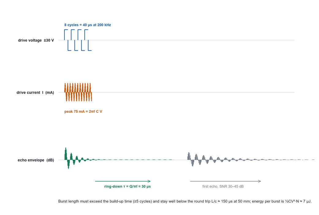
Fig. 5 Drive burst, current and echo envelope. The transmitting element rings for about 48 µs (Q = 30); the first echo must reach the receiving transducer after the ring-down has decayed by 20–30 dB.
5 Common problems and precautions
The eight failures below account for most transducer-related field complaints. They are ordered by frequency, and each is stated as a symptom, a cause and a countermeasure.
5.1 Weak or missing echo after a cable change
Symptom: the meter worked on the bench and reads intermittently in the plant. Cause: the installed lead is longer than the bench lead, so C0 + Ccable has moved and the tuning inductor no longer cancels it; the antiresonance moves by 9 kHz per 2 m and the drive current transfer drops. Precaution: specify the cable length with the transducer, re-tune Lt on site, or use a transducer with an integrated trimmer.
5.2 Poor acoustic coupling and trapped air
Symptom: low amplitude from one transducer only, stable in time. Cause: an air pocket under the matching layer, a dry O-ring, or a face not flush with the bore. At 200 kHz a 0.1 mm air gap presents an impedance discontinuity that reflects more than 99 % of the energy. Precaution: wet the O-ring and the face with the specified coupling fluid, check that the face is flush within 0.2 mm, and verify the echo amplitude against a reference transducer at commissioning.
5.3 Condensation, droplets and fouling
Symptom: a slow, temperature-correlated drift of amplitude, or an intermittent loss after a cold start. Cause: a water film on the face. At 200 kHz the wavelength in water is 7.5 mm and the film behaves as a quarter-wave transformer: 0.5 mm of water detunes the matching layer and changes both amplitude and phase. Precaution: mount the transducers below the pipe axis in wet gas, use a non-wetting PEEK window, and treat the echo amplitude trend as a predictive-maintenance channel rather than as a nuisance.
5.4 Thermal mismatch and cracked matching layer
Symptom: progressive sensitivity loss after thermal cycling, visible as a craze on the face. Cause: the CTE of the epoxy matching layer (40–60 ppm/K) is an order of magnitude above that of the ceramic (5 ppm/K); a 100 K excursion develops enough shear to fatigue the bond. Precaution: use a filled epoxy matched to the ceramic, keep the gas temperature within the transducer rating (or fit a stand-off), and require a −40/+120 °C cycling test at qualification.
5.5 Crosstalk through the wall
Symptom: the receiver detects a pulse before the true echo, or the measured transit time is short and flow-independent. Cause: structure-borne energy travelling through the pipe wall and the spool. Precaution: separate the transducers by at least three body diameters, use a mounting boss that is decoupled from the pipe, and check the received waveform for an early arrival when the pipe is empty.
5.6 Ground loops and EMI
Symptom: noise bursts synchronised with inverter or welding activity, or a 50/100 Hz component in the measured time. Cause: the twisted pair is unscreened and the transducer body floats relative to the electronics. Precaution: bond the housing to the pipe, use a differential receiver with a common-mode choke, and ground the cable screen at the transmitter end only.
5.7 Ageing and drift of the resonance
Symptom: a gradual loss of amplitude over years, with the electrical resonance moving a few kilohertz. Cause: depoling and stress relaxation in the ceramic; the resonance drifts by −0.5 to −2 % per decade of time and the resonance temperature coefficient is about −50 ppm/K. Precaution: include the transducer in the periodic verification (impedance sweep and sensitivity), and keep a spare pair traceable to the original calibration.
5.8 Mechanical damage from pressure cycling
Symptom: a transducer that leaks or that shows a sudden amplitude drop after a pressure surge. Cause: the O-ring extrusion or a fatigue crack in the potting. Precaution: respect the pressure rating with a 1.5 × margin, use a backing ring for the O-ring above 2 MPa, and specify a 10⁵-cycle pressure test for custody service.
6 Applications
The same 200 kHz transducer pair serves four application families, distinguished mainly by gas and pressure rather than by the transducer itself.
· Natural gas custody transfer (5–70 bar). The high density gives an excellent impedance match and a 30–45 dB echo budget on a 60–200 mm path; transducers are wet-in, in spool pieces, with 0.5 % accuracy and a ten-year service life.
· Hydrogen blending. The transducer is unchanged, but the speed of sound rises by 4.7 % for a 10 % H₂ blend, so the meter must be re-verified for the mixture. The transducer face material must be checked for hydrogen permeability if the blend exceeds 20 %.
· Industrial and utility gas (1–10 bar). Compressed air, N₂, O₂, Ar and CO₂ in 25–200 mm lines; often wet or dirty. The transducer is fitted with a protective PEEK window and the coupling is checked at each service.
· Flue gas and combustion air. The gas is hot (100–300 °C) and dusty, so the transducer is fitted with a stand-off and a thermally isolating window; 200 kHz remains usable while the path stays below 200 mm.
Table 3 Application matrix for the 200 kHz transducer pair
Application
Mounting
c (m/s)
L (mm)
Face Ø (mm)
Coupling
Accuracy
Custody CH₄, 5–70 bar
wet-in spool
430–450
60–200
12–18
metal-to-metal, flush
0.5–1.0 %
H₂ blend ≤ 20 %
wet-in spool
460–520
60–120
12–15
flush, welded window
1.0 %
Biogas, wet
bottom-entry
350–420
40–100
12–16
PEEK window, drain
1.5–2.0 %
Compressed air / N₂
clamp-in boss
340–350
30–80
10–15
O-ring, flush
1.0–1.5 %
Flue gas 200 °C
stand-off
400–480
80–200
15–20
thermal break + window
2.0 %
7 Parameter matching in the application
Matching a transducer is not a single calculation but four independent ones — electrical, acoustic, geometric and thermal — and a design that satisfies three of them will still fail in the field.
7.1 Electrical matching: C0, cable and inductor
The transducer presents 2.2 nF to the driver. The cable adds 100 pF/m, the inductor cancels the sum, and the residual reactive current sets the efficiency. The matched values are:
Table 4 Tuning inductor against capacitance (f0 = 200 kHz)
C0 + Ccable
Tuning inductor Lt
Use
1.8 nF (0 m cable)
352 µH
bench test, very short lead
2.2 nF (0 m cable)
288 µH
transducer alone
2.4 nF (2 m cable)
263 µH
typical spool installation
2.6 nF (4 m cable)
243 µH
remote electronics
2.9 nF (7 m cable)
218 µH
limit before the driver loses too much current
3.2 nF (10 m cable)
198 µH
not recommended above 10 m without screening
Lt = 1/((2πf0)²C). A 9 % inductance error leaves about 10 % of the drive current circulating in the capacitance, i.e. −1 dB of echo and increased jitter.
7.2 Acoustic matching: impedance and layer thickness
The matching layer is the only acoustic transformer in the chain, and its tolerance is the tightest in the transducer: λ/4 at 200 kHz is 3.5 mm for an epoxy of cm = 2800 m/s, and a ±0.35 mm error costs 1 dB. The impedance target Zm = √(ZPZT·Zgas) moves with the gas: 0.115 MRayl for air at 1 bar, but 0.19 MRayl for methane at 50 bar. A transducer optimised for atmospheric air is therefore 2–3 dB below optimum in a 50 bar pipeline — a small effect that is nevertheless worth knowing when a transducer is moved between applications.
7.3 Geometric matching: aperture, beam and dead zone
Beam half-angle and dead zone both follow from the face diameter:
θ0 = arcsin(1.22 λ / D) dead zone ≈ 3 Q c / (π f) (7)
A 15 mm face at 200 kHz gives θ0 = 8°, which ensonifies a 25 mm bore at 50 mm separation without touching the wall (Figure 6). The dead zone of 50 mm (3τ at Q = 30) sets the minimum transducer spacing; a shorter spacing needs a lower-Q transducer or a larger frequency. The usual mistake is to enlarge the face to increase sensitivity: the amplitude rises as D², but the beam narrows, the wall echo becomes dominant and the zero stability degrades.
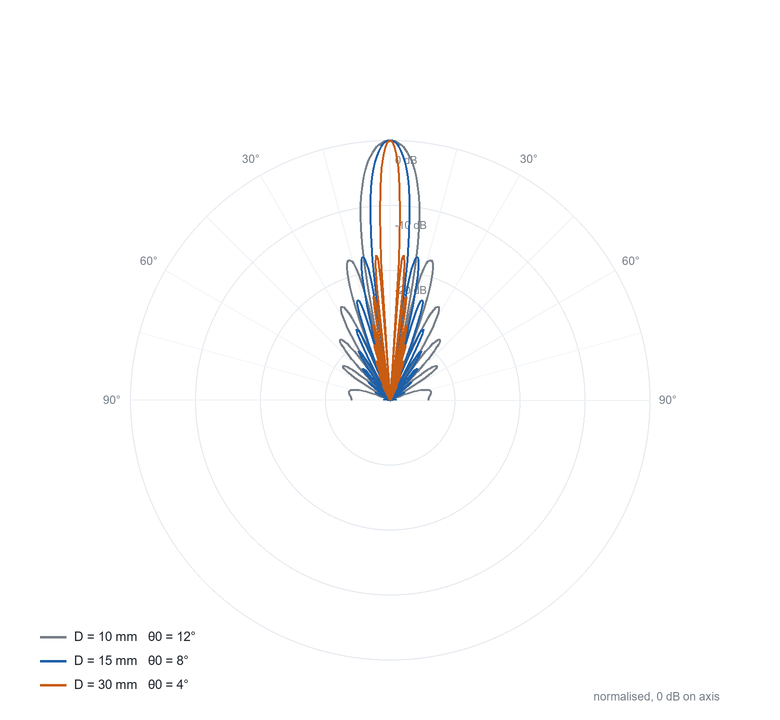
Fig. 6 Directivity of the transducer face at 200 kHz. Fifteen millimetres is the practical optimum for a 25–50 mm bore: wide enough to fill the section, narrow enough to avoid the wall.
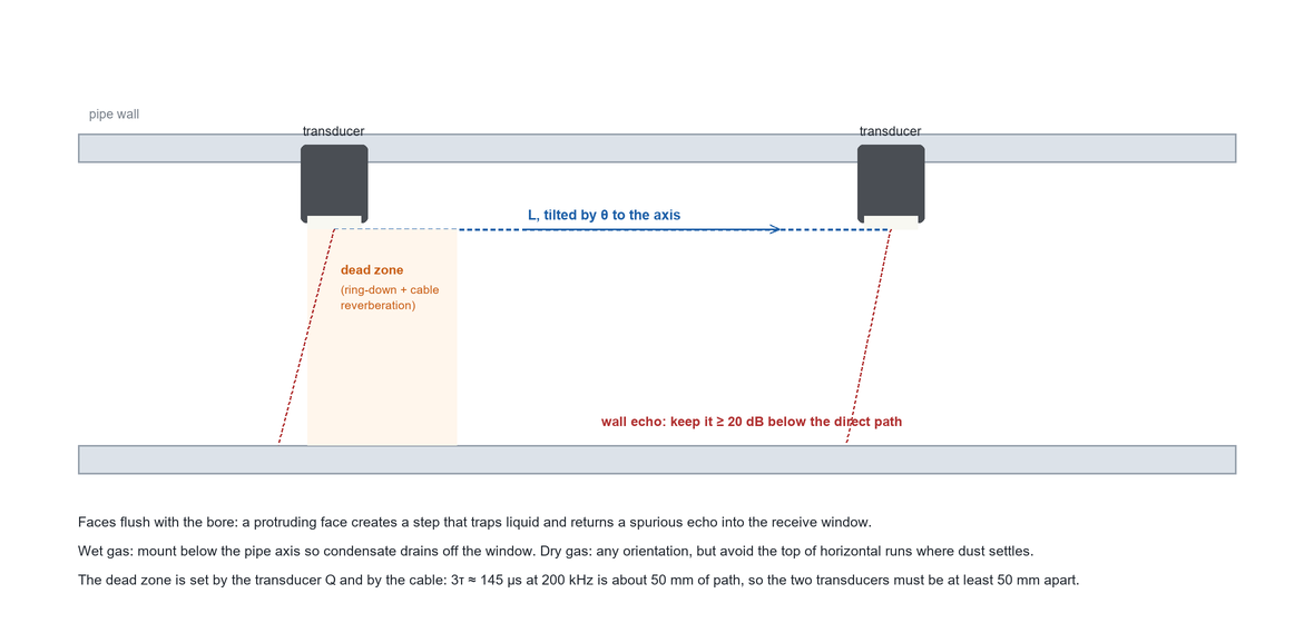
Fig. 7 Installation geometry. The ring-down dead zone and the wall echo, not the electronics, set the minimum path and the transducer spacing.
7.4 Drive and thermal matching
The transducer is a capacitor being driven at resonance, so the drive current is proportional to frequency and capacitance (equation 6). At 30 V and 200 kHz the current is 83 mA; doubling the frequency doubles both the current and the dielectric loss, which is why the same physical transducer rated for 200 kHz cannot simply be driven at 400 kHz. The thermal budget at 200 Hz and 0.8 % duty cycle is dominated by the echo measurement, not by the drive, so the practical limit is dielectric breakdown at about 40 V_rms.
7.5 Receive matching
The receive chain must be matched to the source impedance as well: 2.2 nF at 200 kHz is 0.36 Ω of reactance, so a voltage amplifier sees an almost pure capacitance and its input capacitance adds directly to C0, detuning the transducer exactly as a cable would. A charge amplifier, or a voltage amplifier with <20 pF input capacitance, is therefore the correct front end for a high-impedance piezo transducer.
7.6 Thermal and lifetime matching
The transducer temperature coefficient is small in frequency (−50 ppm/K, 1.2 kHz over 120 K, Figure 8) but not in sensitivity (−0.02 dB/K with a soft peak near 65 °C). For a 0.5 % class meter the sensitivity drift matters only through the AGC and threshold loop, which is why the echo amplitude is logged and used to compensate. Ageing (−0.5 to −2 % per decade) is a long-term term that must be covered by periodic verification rather than by electronics.
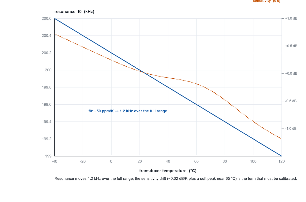
Fig. 8 Resonance and sensitivity against transducer temperature. The resonance shift is benign; the sensitivity drift is the term that enters the measurement through the threshold loop.
8 Acceptance testing
Because the transducer is a passive component, it can be fully characterised without gas flow. Four tests cover the whole specification:
· Impedance sweep (100–300 kHz): confirms f0, Q, C0 and the C0/Cm ratio, and detects a cracked matching layer (broadened resonance) or a shorted element (loss of the motional branch).
· Sensitivity in air at a fixed distance and drive level: the only test that catches a partially detached matching layer; the acceptance window is ±1.5 dB around the reference.
· Electrical insulation and capacitance at 100 V: catches moisture ingress before it becomes a field failure.
· Thermal cycling and pressure cycling: −40/+120 °C, 40 cycles, and 10⁵ pressure cycles at 1.5 × rating; re-measure f0 and sensitivity afterwards and require the drift to stay inside 2 kHz and 1 dB.
Table 5 Transducer failure modes, symptoms and countermeasures
Failure
Symptom
Cause
Countermeasure
Detuning by cable
weak echo, jitter
Lt not re-tuned
match Lt to C0 + Ccable
Trapped air / dry O-ring
low amplitude, one side
impedance break
coupling fluid, flush face
Condensation film
drift with temperature
quarter-wave water layer
bottom-entry, PEEK window
Cracked matching layer
progressive loss
CTE mismatch
filled epoxy, stand-off, cycling test
Wall crosstalk
early pulse, short TOF
structure-borne path
≥3 body diameters separation
Ground loop / EMI
noise bursts, 50/100 Hz
unscreened pair
bond housing, screen one end
Ageing / depoling
slow amplitude loss
stress relaxation
periodic verification
Pressure fatigue
leak, sudden loss
O-ring extrusion
1.5 × margin, backing ring
9 Conclusion
A 200 kHz gas-flow transducer is a small, passive, deliberately simple component whose behaviour is nevertheless fully described by six numbers: f0, Q, C0, Cm, Rm and the matching-layer thickness. Once those are known, the rest of the design follows: Lt = 288 µH for a 2.2 nF transducer, an eight-cycle 30 V burst costing 8 µJ, a 48 µs ring-down that sets a 50 mm dead zone, and a 15 mm face that gives an 8° beam in a 25 mm bore.
The failures that matter in the field are rarely failures of the element itself. They are mismatches: a cable added after the tuning was fixed, an air pocket under the face, a water film in a horizontal line, a wall echo that arrives before the true one. Matching, in the end, is the discipline of keeping four things consistent — electrical, acoustic, geometric and thermal — from the datasheet through the installation.
Because the transducer is also the acoustic reference of the meter, its verification is the meter's verification: an impedance sweep and an air-sensitivity measurement at commissioning, repeated at each service, will catch nearly every degradation path described in §5 before it reaches the reading.
References
[1] ISO 17089-1:2019, Measurement of fluid flow in closed conduits — Ultrasonic meters for gas — Part 1: Meters for custody transfer and allocation measurement.
[2] OIML R137-1:2012, Gas meters — Part 1: Requirements.
[3] ANSI/IEEE Std 176-1987, IEEE Standard on Piezoelectricity (constitutive equations, d, g, k constants).
[4] L. C. Lynnworth, Ultrasonic Measurements for Process Control, Academic Press, 1989 — chapters on piezoelectric transducers and matching layers.
[5] L. C. Lynnworth and Y. Liu, “Ultrasonic flowmeters: half-century progress report, 1955–2005”, Ultrasonics 44 (2006) e1371–e1378.
[6] P. Hauptmann, N. Hoppe and A. Püttmer, “Application of ultrasonic sensors in the process industry”, Measurement Science and Technology 13 (2002) R73–R83.
[7] R. W. Rittenmyer, “Electroceramic transducers for ultrasonic flow measurement”, Ferroelectrics (review of resonance modes and impedance behaviour of PZT discs).
[8] IEEE Std 177-1966, Standard Definitions and Methods of Measurement for Piezoelectric Vibrators (resonance/antiresonance measurement, Q determination).
[9] O. Cramer, “The variation of the specific heat ratio and the speed of sound in air with temperature, pressure, humidity, and CO₂ concentration”, JASA 93 (1993) 2510–2516.
[10] ISO 9613-1:1993, Acoustics — Attenuation of sound during propagation outdoors — Part 1: Calculation of the absorption of sound by the atmosphere.
[11] ams AG, TDC-GP30 and Texas Instruments, TDC7200 data sheets — time-to-digital converters used with 200 kHz transducers.
- Previous:How to select variable reluctance resolver
- Next:Already the last article
Links:Service Hotline
+86 13923792185
Website:www.micmetering.com
Address:6th Floor, Block B, Area A, Qinghu Science and Technology Park, Longhua District, Shenzhen, Guangdong Province
Copyright © 2025 MIC Metering (Shenzhen) Limited 粤ICP备2025358196号-1 Cookies Policy-
Service Hotline
Service Hotline
+86 13923792185
-
WeChat

-
TOP
Our Cookie Usage Policy
Our website uses cookies and other similar technologies to distinguish you from other users of our website. This helps us provide you with a good experience when you browse our website and allows us to improve our website. For more information, please refer to our Cookie Policy. - About Us